Examples

In this section, we provide example code to show how to fit flexTPC with various methodologies (least squares estimation, maximum likelihood estimation and Bayesian approaches).

Plotting flexTPC curves

First, we provide code that implements the flexTPC model. There are two different parametrizations of flexTPC that can be useful in different circumstances (see paper for details).

# FlexTPC model for thermal performance curves.
# (parametrized with alpha/beta)
flexTPC <- function(temp, Tmin, Tmax, rmax, alpha, beta) {
  s <- alpha * (1 - alpha) / beta^2
  result <- rep(0, length(temp))
  Tidx = (temp > Tmin) & (temp < Tmax)
  result[Tidx] <- rmax * exp(s * (alpha * log( (temp[Tidx] - Tmin) / alpha) 
                  + (1 - alpha) * log( (Tmax - temp[Tidx]) / (1 - alpha)) 
                  - log(Tmax - Tmin)) ) 
  return(result)
}
  
# FlexTPC model for thermal performance curves.
# (parametrized with Topt/B)
flexTPC2 <- function(temp, Tmin, Tmax, rmax, Topt, B) {
  alpha <- (Topt - Tmin) / (Tmax - Tmin)
  beta <- B / (Tmax - Tmin)
  if((alpha >= 0.0) & (alpha <= 1.0)) {
    return(flexTPC(temp, Tmin, Tmax, rmax, alpha, beta))
  } else {
    return(rep(0, length(temp)))
  }
}

These functions are written in a slightly different way as the form of the equation shown in the paper that tends to be more numerically stable.Let’s plot some flexTPC curves.

# Creates a vector of temperatures from 5 to 38°C with a 0.1°C step.
temp <- seq(5, 38, 0.1)

par(mfrow=c(1,1))
# Plots a flexTPC curve using the alpha/beta parametrization.
plot(temp, flexTPC(temp, Tmin=10, Tmax=35, rmax=1.0, alpha=0.8, beta=0.2), type='l',
     xlab='Temperature [°C]', ylab='Trait performance', lwd=2)

# Plots a flexTPC curve using the Topt/B parametrization.
# We are intentionally picking a Topt that is a little lower than the previous
# curve so they are not plotted on top of each other.
lines(temp, flexTPC2(temp, Tmin=10, Tmax=35, rmax=1.0, Topt=29.0, B=5.0),
      col='red', lwd=2)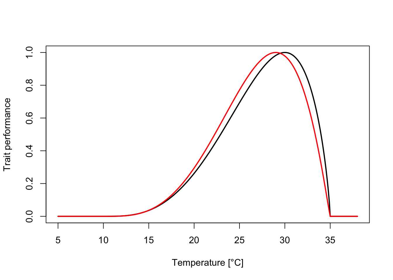

At this point, you may want to try modifying the parameter values to observe how this changes the curve. This can be a useful way to get intuition on what the parameters are doing to the curve and can be a good way to find reasonable starting values for the model parameters when fitting data.

Fitting thermal performance curves

Here we include some examples that show how to fit flexTPC to real data. To follow along these examples, please download the datasets provided here.

When fitting a thermal performance curve model (e.g. flexTPC) to data, our goal is to find the model parameters that are most consistent with the observations. In statistics, curve fitting problems similar to this are referred to as regression problems. More specifically, this is a parametric nonlinear regression, where the regression function that is used is the TPC model.

There are different methods that can be used to estimate parameters in a regression problem.

• Least squares estimation is a simple method that is popular in practice.

• Maximum likelihood estimation allows modeling the data with different probability distributions, and optionally allows modeling the error distribution to better account for non-constant variance.

• Bayesian approaches use probability distributions to describe parameter uncertainty. These methods allow incorporating external information (e.g. from other experiments or the habitat of the organism) to constrain model parameters when estimating TPCs. They can also incorporate different probability distributions and account for non-constant variance.

In these examples, we purposefully use slightly different modeling approaches than those we follow in the paper to illustrate how to deal with different kinds of data (e.g. to account for non-constant variance) and to provide code that uses different assumptions in addition to the code used for the analyses in the paper.