A simple approach to estimate thermal performance curves (TPCs) is to perform nonlinear least squares estimation. This finds the curve that minimizes the squared difference between the TPC and the data points.
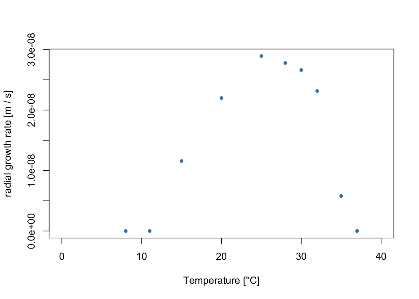
In this example, we will fit the flexTPC model to data of the radial growth rates of the fungus Metarhizium anisopliae. This data is originally from Ouedraogo et al 1997 and was digitized by Kontopoulos et al 2024.
Let’s start by reading in the data and plotting it.
data <-read.csv('TPC_data_examples.csv') # From Kontopoulos et al.data <-subset(data, data$id ==39697) # Subset Ouedraogo et al dataset.plot(data$temperature, data$trait_value, xlim=c(0, 40),xlab='Temperature [°C]', ylab='radial growth rate [m / s]',pch=20, col='steelblue')
In order to fit flexTPC to this data, we will need to code the model equation and an error function that calculates the squared difference between a curve and the data points.
# FlexTPC model for thermal performance curves.# (parametrized with alpha/beta)flexTPC <-function(temp, Tmin, Tmax, rmax, alpha, beta) { s <- alpha * (1- alpha) / beta^2 result <-rep(0, length(temp)) Tidx = (temp > Tmin) & (temp < Tmax) result[Tidx] <- rmax *exp(s * (alpha *log( (temp[Tidx] - Tmin) / alpha) + (1- alpha) *log( (Tmax - temp[Tidx]) / (1- alpha)) -log(Tmax - Tmin)) ) return(result)}# Returns a function that calculates the squared error between data and a flexTPC curve.get_sq_err_fn <-function(temp, y, lower.bounds, upper.bounds) {# temp: Vector of measured temperature values.# y: Vector of measured performance values.# lower_bounds, upper_bounds: Lower and upper bounds for the parameters. f <-function(par) {# Return infinity (worst possible error) if parameters are outside of chosen# upper and lower bounds.if((sum(par < lower.bounds) +sum(par > upper.bounds)) >0) {return(Inf) } else {# Otherwise return squared difference between data and flexTPC curve.return(sum((y -flexTPC(temp, par[1], par[2], par[3], par[4], par[5]))^2)) } }return(f) }
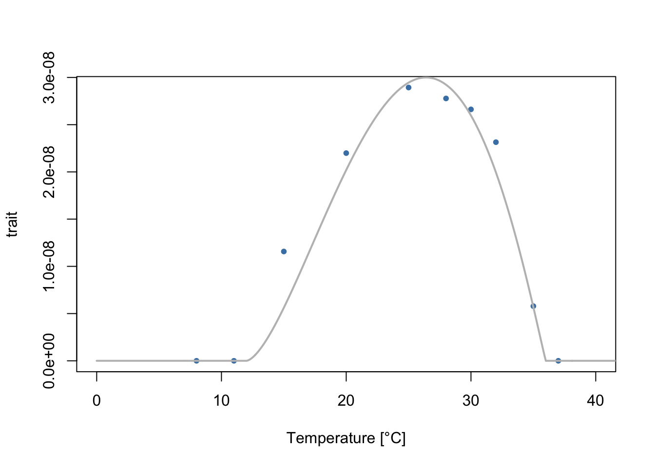
We also need an initial guess for the parameters for the flexTPC model. We will input these initial parameters and the error function to minimize into the function in R. The intuitive parameters of the flexTPC model make it simple to choose reasonable starting parameter values.
Let’s pick some initial values and plot the data and a flexTPC curve with initial guesses for the parameters (picked visually).
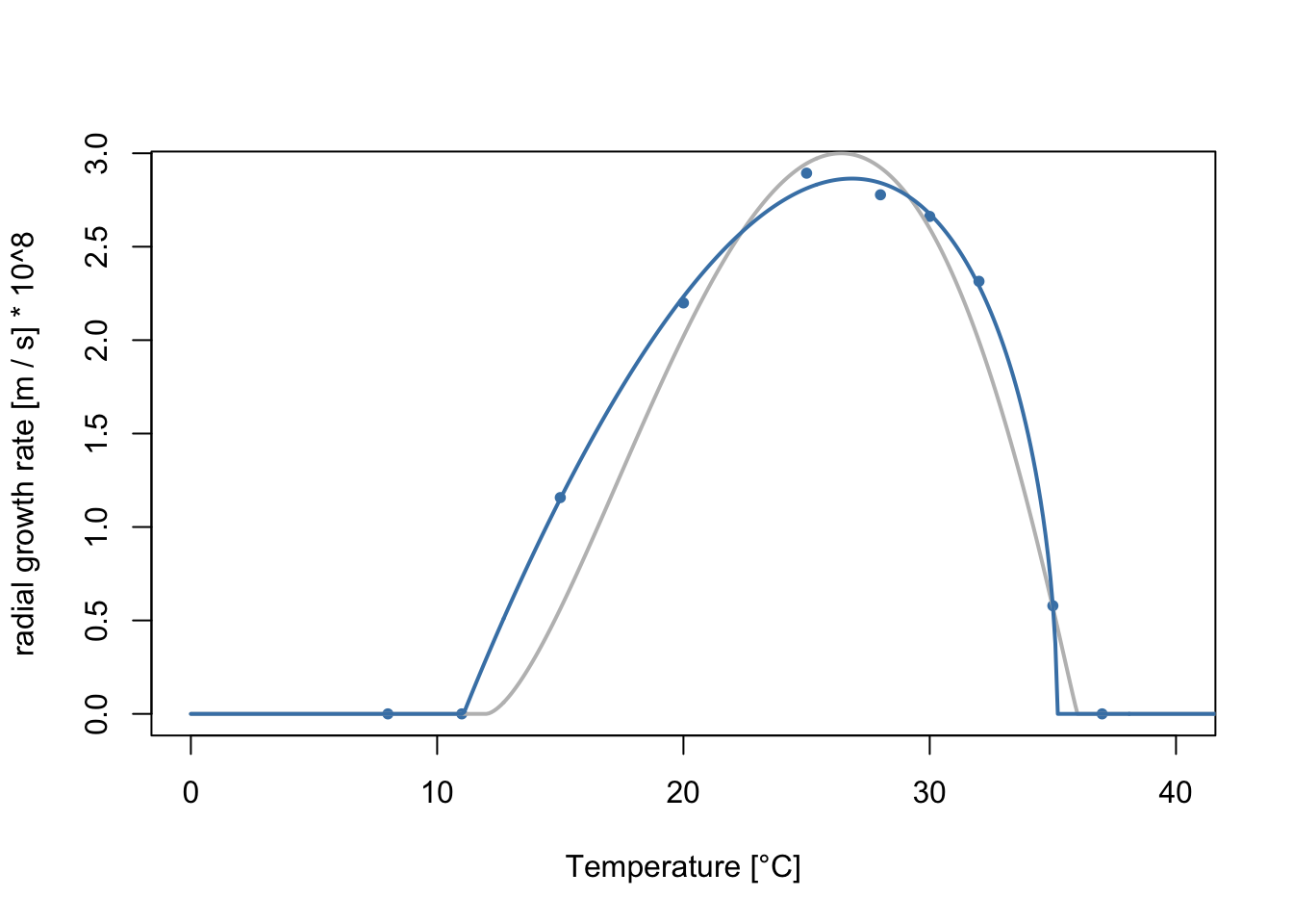
We will now find the parameters that minimize the squared error to our data. Before doing so, it is convenient to change the units of the data to help the optimization algorithm (as it sometimes has trouble if the parameters to optimize are of very different orders of magnitude). Let’s do this and fit the curves.
temp <- data$temperaturey <- data$trait_value *10^8# Convert units of the trait value data so they are close to unit scale.init.par <-c(12, 36, 3, 0.6, 0.3)names(init.par) <-c("Tmin", "Tmax", "rmax", "alpha", "beta")# Lower and upper bounds for the parameters.lower.bounds <-c(0, 30, 0, 0.1, 0.1)upper.bounds <-c(15, 45, 10, 0.9, 0.7)f <-get_sq_err_fn(temp, y, lower.bounds, upper.bounds) # Get error function with the chosen bounds of the parameters.fit <-optim(init.par, f, control=list(maxit=10000))
Finding the optimal temperature and approximate thermal breadth
The optimum temperature \(T_\mathrm{opt}\) of a flexTPC curve can be calculated with the following equation:
\[T_{\mathrm{opt}} = \alpha T_\max + (1- \alpha) T_\min\] and the approximate thermal breadth \(B\) at 88% of the maximum performance with the equation \[ B = \beta (T_\max - T_\min)\] We can use these equations to find the least square estimates for \(T_\mathrm{opt}\) and \(B\).
B <- fit$par['beta'] * (fit$par['Tmax'] - fit$par['Tmin'])names(B) <-'B'B
       B
9.330535
Finding the thermal breadth at other reference values
In many applications, researchers may be interested on the thermal breadth at a different reference performance value than 88%. We provide an algorithm to find the temperatures corresponding to any performance numerically from the flexTPC model. This can be used to find the least square estimate of the thermal breadth at any desired performance value (or more accurately at 88%). As an input, our algorithm takes the parameters of a flexTPC curve and a reference relative performance level \(w_\mathrm{ref}\), expressed as a percentage of the maximum trait performance. For example, finding the temperatures with \(w_\mathrm{ref}=0.5\) corresponds to the half-maximum temperatures, or \(w_\mathrm{ref}=0.8\) to the temperatures where performance is 80% of the maximum.
## f1 and f2 are auxiliary functions used by our algorithm.f1 <-function(tau, wref, alpha, s) { logf1 <-log(alpha) + (1/ (alpha * s) ) *log(wref) + ((1- alpha) / alpha) * (log(1- alpha) -log(1- tau))return(exp(logf1))}f2 <-function(tau, wref, alpha, s) { B <-log(1- alpha) + (1/ ((1- alpha) * s) ) *log(wref) + (alpha / (1- alpha)) * (log(alpha) -log(tau))return(1-exp(B))}flexTPC_nd_roots <-function(wref, alpha, beta, tol=1e-6) {## Implements fixed point algorithm to find nondimensional temperatures tau1, ## tau2 corresponding to a specific wref in a flexTPC model.## tol: Error tolerance for tau1, tau2 (nondimensional temperatures where## performance is wref).## alpha, beta: Parameters for flexTPC curve. s <- alpha * (1- alpha) / beta^2 tau1 <- alpha /2 tau2 <- alpha + (1- alpha) /2 err <-Infwhile(err > tol) { new_tau1 <-f1(tau1, wref, alpha, s) new_tau2 <-f2(tau2, wref, alpha, s) err <-pmax(abs(tau1 - new_tau1), abs(tau2 - new_tau2)) tau1 <- new_tau1 tau2 <- new_tau2 }return(c(tau1, tau2))}flexTPC_roots <-function(wref, Tmin, Tmax, alpha, beta, tol=1e-6) {## Finds (dimensional) temperatures T1, T2 corresponding to a specific wref## in a flexTPC model.## Does this by finding nondimensional temperatures and converting them to## dimensional temperatures.## tol: Error tolerance for tau1, tau2 (nondimensional temperatures where performance is wref).## alpha, beta: Parameters for flexTPC curve. nd_roots <-flexTPC_nd_roots(wref, alpha, beta, tol=tol)return(Tmin + nd_roots*(Tmax - Tmin))}
Let’s find the half-maximum temperatures and thermal breadth.
Researchers may be interested on quantifying the uncertainty in the estimated model parameters. In frequentist statistics, this uncertainty arises because the data we have is random, and if we were to hypothetically repeat the experiments and data collection we’d get slightly different measurements (and therefore different TPC estimates when fitting the curve!).
One general approach to construct confidence intervals is bootstrapping, a procedure based on data resampling. The most common approach is a nonparametric bootstrap, in which construct many bootstrap samples by sampling our original \(N\) datapoints to get a new dataset of the same size. In these bootstrap samples some observations will be repeated and some will be missing, so each sample will be different than our original dataset. We can then fit the model to each of these bootstrap samples, and keep track of the estimated model parameters. We can then construct confidence intervals from the distribution of the parameters for the individual bootstrap sample estimates.
## Performs a nonparametric boostrap to get confidence intervals of model parameters.set.seed(42) # Set seed for reproducibility# Number of bootstrap samples# Note: You can make this small for testing (so the code runs faster), but# should be at least 10000 for real applications.N <-10000# Matrix to store bootstrap resultsbts_samples <-matrix(nrow=N, ncol=9)temp <- data$temperature# Change scale of trait values to be close to unit scale to help optimization.y <- data$trait_value *10^8n.obs <-length(temp)init.par <-c(12, 36, 3, 0.6, 0.3)lower.bounds <-c(0, 30, 0, 0.1, 0.1)upper.bounds <-c(15, 45, 10, 0.9, 0.7)for(i in1:N) {# Sample observations with replacement sample.idx <-sample(1:n.obs, n.obs, replace=TRUE)# Get function to calculate error from current bootstrap sample. f <-get_sq_err_fn(temp[sample.idx], y[sample.idx], lower.bounds, upper.bounds)# Fit flexTPC curve to current bootstrap sample. sample.fit <-optim(init.par, f, control=list(maxit=100000))# Store estimated flexTPC parameters for current boostrap sample. bts_samples[i, 1:5] <- sample.fit$par}
We can now find confidence intervals for the model parameters (and also other quantities derived from them, like \(T_\mathrm{opt}\) and \(B\), or the half-maximum temperatuers). We can get a boostrap estimate for these quantites by transforming our bootstrap samples for the model parameters as appropriate.
[1] Ouedraogo, A., J. Fargues, M.S. Goettel, and C.J. Lomer. 1997. “Effect of Temperature on Vegetative Growth among Isolates of Metarhizium Anisopliae and M. Flavoviride.” Mycopathologia 137 (1): 37–43. https://doi.org/10.1023/a:1006882621776.
[2] Kontopoulos, Dimitrios - Georgios, Arnaud Sentis, Martin Daufresne, Natalia Glazman, Anthony I. Dell, and Samraat Pawar. 2024. “No Universal Mathematical Model for Thermal Performance Curves across Traits and Taxonomic Groups.” Nature Communications 15 (1). https://doi.org/10.1038/s41467-024-53046-2.